Images and Demos for:

Multi-Resolution computation and presentation of Contour Trees

(PDF paper).

Demos for Microsoft Windows and for Linux:

Click on the images below to download the corresponding demo.
For Windows: Unzip the archive. For Linux: tar xvzf filename.tar.gz
Enter in the new directory created and double click on "RUNME.bat" (Windows) or execute "RUNME" (Linux)
Press the space-bar to load the next precomputed scene parameters.
Press shift-space-bar to load the previous precomputed scene parameters.
Follow the "Complete demo instructions" below to set up your own view.

2D Examples

Dinosaur

Hippopotamus

Elephant

Cow

3D Examples

Electron density
distribution

Neghip

Silicium

Fuel

Complete demo instructions

Main Window

This windows shows the embedded contour tree, the level set for the actual isovalue, the mesh (only for 2D meshes, not for volumetric grids) and the actual selected values (see top and bottom black bars)

left mouse button click & drag	rotate the scene
[SHIFT] + left mouse button click & drag (along the X axis)	zoom in, zoom out the scene
middle mouse button click & drag	change the pan of the actual scene
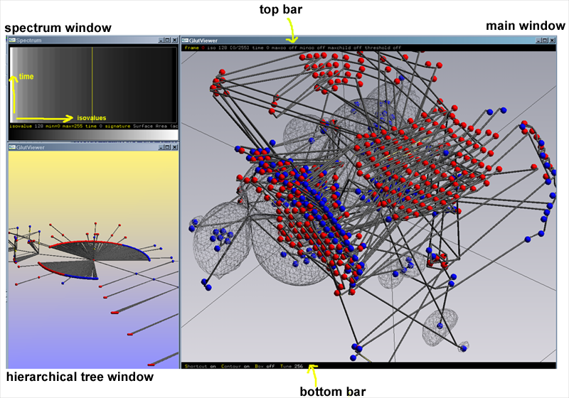
[left] [right] keyboard arrows	Switch for the change of a specific value: (see highlighted item on the main window top bar): frame, isovalue, time, max overall, min overall, max number of children, threshold
[up] [down] keyboard arrows	change the current value, up increases it, down decreases it (to set the"sensibility" of the change use 't' and 'T')
'g'	change the view mode of the embedded contour three
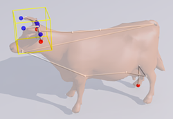
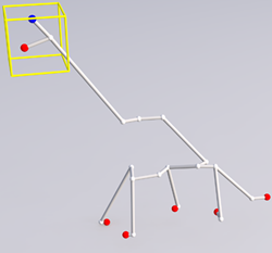
'B'/'b'	enable/disable or increase/decrease the size of the bounding box which specifies the current region of interest
'm'	Only for triangular mesh. Change the view mode of the current mesh
'c'	enable/disable or change the view mode of the level sets of the actual dataset
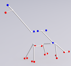
'R'/'r'	increase/decrease the radius of the spheres of the contour trees
'D'/'d'	increase/decrease the radius of the cylinders of the contour trees
's'	save the current frame or enable/disable shortcut
'o'	open the current frame if the highlighted item is "frame" in the top bar. otherwise set to 'off' the filter for maximum overall, minimum overall, threshold or max number of children

Hierarchical Contour Tree Window

This windows shows the hierarchical contour tree using the orrery-like layout

left mouse button click & and drag	rotate the scene
[SHIFT] + left mouse button click & drag (along the X axis)	zoom in, zoom out the scene
middle mouse button click & drag	change the pan of the actual scene
'g'	change the view mode of the hierarchical contour three
'X'/'x'	scale (increase or decrease) the space occupancy along the X axis
'Y'/'y'	scale (increase or decrease) the space occupancy along the Y axis
'Z'/'z'	scale (increase or decrease) the space occupancy along the Z axis

Spectrum window

The X axis displays isovalues, the Y axis displays the time.

left mouse button click	change the isovalue and the actual time
right mouse button click & drag	zoom on a particular area of the spectrum
middle mouse button click	change the current palette
'0'..'4'	change the signature (surface area, min volume, max volume, gradient)
'b'	display the spectrum of the entire dataset (disable any actual zoom)

Gallery

Electron density distribution

Contour Tree at three levels of resolution for the electron density distribution rho computed with an ab initio simulation for water molecules at high pressure.

At coarse scale (top) the tree has only one maximum (blue sphere) per water molecule. At medium scale (middle) the topology reconstructs one dipole per molecule with one maximum and one minimum (red sphere). At fine scale (bottom) only the noise is removed and three extrema per molecule reconstruct each atom in the simulation.

Adaptive refinement in the area marked with a rectangle (middle) can be used to refine the topology for two particular molecules. This is shown on the right at coarse, medium and fine scale both for the Contour Tree and for the embedding (shown side by side)

2D Triangulated Models

Here we show some examples of the computation of contour trees for 2D meshes. In the first column we show the original model. In the second column the Complete Contour Trees are drawn with their critical points in their original position (the Morse function f is the height in the vertical direction). In the third column the full topology is shown only in the bounding box containing the head of the model (using the adaptive refinement of our multi-resolution representation).

Neghip dataset

Neghip dataset representing the spatial probability distribution of the electrons in a high potential protein molecule.

In the figure you can see: (top row) level sets for different isovalues; (bottom left) Contour Tree of the full topology; (bottom middle) Contour Tree of the coarse resolution topology; (bottom right) critical points of the coarse scale topology, displayed together with a semi transparent level set.

Silicium grid

Topology of the electron density distribution in a simulation of a silicium grid.

The topology can be presented incrementally from coarse (left) to fine (right).